Model masking

This tutorial explores some of ramannoodle’s masking features. These features are useful when analyzing simulated Raman spectra.

InterpolationModel, as well it’s subclasses (such as ARTModel), can be modified by “masking” specified degrees of freedom (DOFs). When a DOF is masked, it is excluded when calculating polarizabilities and therefore will not be accounted for when calculating Raman spectra. Raman spectra computed with masking should be regarded as partial Raman spectra. By choosing the masks wisely, quite a bit can be learned about which atom (or groups of atoms) correspond to which features in the simulated Raman spectra.

First, our usual imports.

import numpy as np
from matplotlib import pyplot as plt
import matplotlib_inline

matplotlib_inline.backend_inline.set_matplotlib_formats('png')
plt.rcParams['figure.dpi'] = 300
plt.rcParams['font.family'] = 'sans-serif'
plt.rcParams["mathtext.default"] = 'regular'
plt.rcParams['axes.linewidth'] = 0.5
plt.rcParams['xtick.major.width'] = 0.5
plt.rcParams['xtick.minor.width'] = 0.5
plt.rcParams['lines.linewidth'] = 1.5

import ramannoodle as rn

Setup of model

We will be computing TiO2’s Raman spectrum using data available in tests/data/TiO2 (see Github repo). We will be basing this spectrum on frozen phonon calculations and use ARTModel to estimate polarizabilities.

data_dir = "../../../test/data/TiO2"
# phonon_OUTCAR contains phonons (duh) as well as the reference TiO2 structure.
phonon_outcar = f"{data_dir}/phonons_OUTCAR"

# Read the phonons
phonons = rn.io.vasp.outcar.read_phonons(phonon_outcar)
# Read the reference structure. This might take a few moments...
ref_structure = rn.io.vasp.outcar.read_ref_structure(f"{data_dir}/ref_eps_OUTCAR")

# We'll need the polarizability of the reference structure.
_, ref_polarizability = rn.io.vasp.outcar.read_positions_and_polarizability(
   f"{data_dir}/ref_eps_OUTCAR"
)
model = rn.pmodel.ARTModel(ref_structure, ref_polarizability)

# OUTCARS are polarizability calculation where atom 5 (Ti)
# was displaced +0.1 and +0.2 angstrom in the x direction
model.add_art_from_files(
    [f"{data_dir}/Ti5_0.1x_eps_OUTCAR"], file_format = 'outcar'
  )
model.add_art_from_files(
    [f"{data_dir}/Ti5_0.1z_eps_OUTCAR"],file_format = 'outcar'
  )
model.add_art_from_files(
    [f"{data_dir}/O43_0.1z_eps_OUTCAR", f"{data_dir}/O43_m0.1z_eps_OUTCAR"],
    file_format="outcar"
)
model.add_art_from_files(
    [f"{data_dir}/O43_0.1x_eps_OUTCAR"], file_format = 'outcar'
)
model.add_art_from_files([f"{data_dir}/O43_0.1y_eps_OUTCAR"],file_format = 'outcar')
model

╭──────────────┬─────────────────────────────────────────────┬─────────────┬────────────────────╮
│   Atom index │ Directions                                  │ Specified   │   Equivalent atoms │
├──────────────┼─────────────────────────────────────────────┼─────────────┼────────────────────┤
│            0 │ [-1. -0. +0.], [-0. -1. -0.], [-0. -0. +1.] │ 3/3         │                 35 │
│           36 │ [+0. +0. +1.], [+1. +0. +0.], [+0. +1. +0.] │ 3/3         │                 71 │
╰──────────────┴─────────────────────────────────────────────┴─────────────┴────────────────────╯

All degrees of freedom have been specified. We are now ready to do some Raman calculations!

Calculating the full Raman spectrum

# Compute and plot spectrum
spectrum = phonons.get_raman_spectrum(model)
wavenumbers, total_intensities = spectrum.measure(
    laser_correction = True,
    laser_wavelength = 532,
    bose_einstein_correction = True,
    temperature = 300
)
wavenumbers, total_intensities = rn.spectrum.utils.convolve_spectrum(wavenumbers, total_intensities)
fig = plt.figure(constrained_layout = True, figsize = (8, 3))
axis = fig.add_subplot(111)
axis.plot(wavenumbers, total_intensities)
axis.set_ylabel("Intensity (a.u.)")
l = axis.set_xlabel(r"Raman shift ($\mathregular{cm^{-1}}$)")

Isolating atomic contributions

One question we could ask is which parts of the Raman spectrum are associated with motion of Ti atoms and which parts are associated more with O atoms. In this case, we can produce two masked ARTModel’s, one with the Ti atoms masked and other with the O atoms masked.

fig = plt.figure(constrained_layout = True, figsize = (8, 4))
axis = fig.add_subplot(111)

total_model = model
O_dof_indexes = total_model.get_dof_indexes('O')
Ti_model = total_model.get_masked_model(O_dof_indexes) # Mask O to leave only Ti
Ti_dof_indexes = total_model.get_dof_indexes('Ti')
O_model = total_model.get_masked_model(Ti_dof_indexes) # Mask Ti to leave only O

offset = 0
models = [Ti_model, O_model, total_model]
labels = ['Ti contribution', 'O contribution', 'Total spectrum']
for plot_model, label in zip(models, labels):

    spectrum = phonons.get_raman_spectrum(plot_model)
    wavenumbers, intensities = spectrum.measure(
        laser_correction = True,
        laser_wavelength = 532,
        bose_einstein_correction = True,
        temperature = 300
    )
    wavenumbers, intensities = rn.spectrum.utils.convolve_spectrum(wavenumbers, intensities)
    axis.plot(wavenumbers, intensities + offset, label = label)
    offset += np.max(intensities) + 0.02

axis.set_ylabel("Intensity (a.u.)")
axis.set_xlabel(r"Raman shift ($\mathregular{cm^{-1}}$)")
axis.set_yticks([])
l = axis.legend()

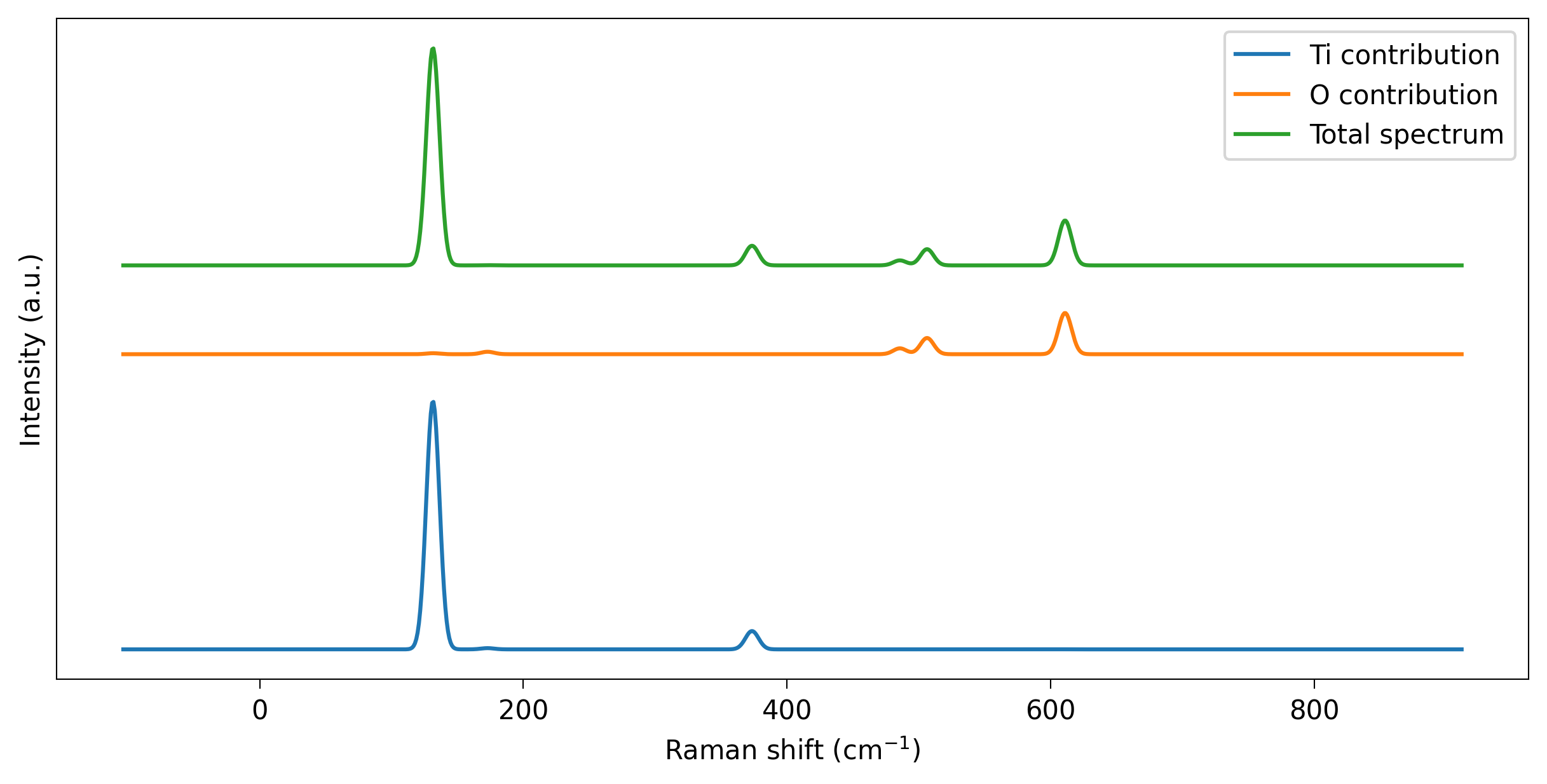
Convince yourself that this makes sense. Hint: consider the vibrational frequencies of the heavier Ti atoms vs the lighter O atoms.

Although this a very simple example, model masking is extremely powerful. By isolating the influence of individual atomic motions on the Raman spectrum, we can gain deep insight into the factors regulating the Raman shifts and Raman intensities of certain motions. In addition, masking gives us a straightforward way to isolate the Raman spectra of specific atoms or groups of atoms. This is useful in many cases, for example when considering defects.

Pitfalls

It is important of a model’s mask, lest you unintentionally use a masked model and believe the results represent the total spectrum. You can check a model’s masking status using its __repr__ string:

print(repr(O_model))

# OR (in Jupyter notebooks)
O_model

╭──────────────┬─────────────────────────────────────────────┬─────────────┬────────────────────╮
│   Atom index │ Directions                                  │ Specified   │   Equivalent atoms │
├──────────────┼─────────────────────────────────────────────┼─────────────┼────────────────────┤
│            0 │ [-1. -0. +0.], [-0. -1. -0.], [-0. -0. +1.] │ 3/3         │                 35 │
│           36 │ [+0. +0. +1.], [+1. +0. +0.], [+0. +1. +0.] │ 3/3         │                 71 │
╰──────────────┴─────────────────────────────────────────────┴─────────────┴────────────────────╯
  ATTENTION: 108/324 atomic Raman tensors are masked. 

╭──────────────┬─────────────────────────────────────────────┬─────────────┬────────────────────╮
│   Atom index │ Directions                                  │ Specified   │   Equivalent atoms │
├──────────────┼─────────────────────────────────────────────┼─────────────┼────────────────────┤
│            0 │ [-1. -0. +0.], [-0. -1. -0.], [-0. -0. +1.] │ 3/3         │                 35 │
│           36 │ [+0. +0. +1.], [+1. +0. +0.], [+0. +1. +0.] │ 3/3         │                 71 │
╰──────────────┴─────────────────────────────────────────────┴─────────────┴────────────────────╯
  ATTENTION: 108/324 atomic Raman tensors are masked. 

If in doubt, you can always use unmask to remove the mask.

O_model.unmask()
O_model

╭──────────────┬─────────────────────────────────────────────┬─────────────┬────────────────────╮
│   Atom index │ Directions                                  │ Specified   │   Equivalent atoms │
├──────────────┼─────────────────────────────────────────────┼─────────────┼────────────────────┤
│            0 │ [-1. -0. +0.], [-0. -1. -0.], [-0. -0. +1.] │ 3/3         │                 35 │
│           36 │ [+0. +0. +1.], [+1. +0. +0.], [+0. +1. +0.] │ 3/3         │                 71 │
╰──────────────┴─────────────────────────────────────────────┴─────────────┴────────────────────╯