Basics

This notebook (available on Github) contains a short tutorial showcasing ramannoodle’s workflow and basic capabilities.

We’ll begin with some imports, plus some customizations to matplotlib.

import numpy as np
from matplotlib import pyplot as plt
import matplotlib_inline

matplotlib_inline.backend_inline.set_matplotlib_formats('png')
plt.rcParams['figure.dpi'] = 300
plt.rcParams['font.family'] = 'sans-serif'
plt.rcParams["mathtext.default"] = 'regular'
plt.rcParams['axes.linewidth'] = 0.5
plt.rcParams['xtick.major.width'] = 0.5
plt.rcParams['xtick.minor.width'] = 0.5
plt.rcParams['lines.linewidth'] = 1.5

import ramannoodle as rn

We will be computing TiO2’s Raman spectrum using data available in tests/data/TiO2 (see Github repo). We will be basing this spectrum on frozen phonon calculations and use InterpolationModel to estimate polarizabilities.

Setup

First, we will read in phonons.

data_dir = "../../../test/data/TiO2"
phonon_outcar = f"{data_dir}/phonons_OUTCAR"

# Read the phonons
phonons = rn.io.vasp.outcar.read_phonons(phonon_outcar)

Then we’ll read in a reference structure and start building our polarizability model.

# Read a reference (minimum) structure.
ref_structure = rn.io.vasp.outcar.read_ref_structure(f"{data_dir}/ref_eps_OUTCAR")

# We'll need the polarizability of the minimum structure.
_, ref_polarizability = rn.io.vasp.outcar.read_positions_and_polarizability(
   f"{data_dir}/ref_eps_OUTCAR"
)
model = rn.pmodel.InterpolationModel(ref_structure, ref_polarizability)

# Using __repr__, we can check out model.
model

InterpolationModel with 0/324 degrees of freedom specified.

We’ve set up model, but we are not yet ready to use it to predict polarizabilities. The __repr__ string of the model indicates that we haven’t specified any of the 324 degrees of freedom in this system. To specify these, we’ll need to add data! Specifically, we will walk through the system’s symmetrically distinct degrees of freedom and add relevant polarizabilities for displacements along those degrees of freedom.

Building up our model

You can find the TiO2 supercell we’re using for these calculations at tests/data/TiO2/POSCAR. Note that there are only two symmetrically distinct atoms - one Ti and one O. If we understand how movement of an atom influences the polarizability, we can use symmetry to derive the behavior of those that are symmetrically equivalent.

Let’s focus on a single Ti atom: atom 5 in our structure. Visualize the POSCAR mentioned above, for example using VESTA. Think about displacing atom 5 along the x-axis. Convince yourself that displacements in the +x direction can be related by symmetry to displacements in the -x direction. These displacements symmetrically equivalent.

Atom 5’s displacement along the x-axis is a degree of freedom (DOF) of the system. Convince yourself that TiO2 structure contains many DOFs that are symmetrically equivalent to this DOF.

InterpolationModel’s key assumption is that every DOF modulates the polarizability independently. The module estimates this modulation using an interpolation around each DOF. We need to “add” each DOF to model, specifying specific displacements as well as polarizabilities for these displacements (which we calculate using VASP). Internally, the model will handle all symmetry considerations.

# OUTCARS are polarizability calculation where atom 5 (Ti)
# was displaced +0.1 and +0.2 angstrom in the x direction
model.add_dof_from_files(
    [f"{data_dir}/Ti5_0.1x_eps_OUTCAR", f"{data_dir}/Ti5_0.2x_eps_OUTCAR"],
    file_format = 'outcar', interpolation_order=2
)

# (36 equivalent Ti atoms) * (2 equivalent directions) --> 72 dofs should be added
model

InterpolationModel with 72/324 degrees of freedom specified.

We’ve added a total of 72 interpolations (i.e. 72 DOFs). Convince yourself that this makes sense.

# atom 5 moving +0.1 and +0.2 angstroms in the z direction
model.add_dof_from_files([f"{data_dir}/Ti5_0.1z_eps_OUTCAR",
                          f"{data_dir}/Ti5_0.2z_eps_OUTCAR"],
                         file_format = 'outcar', interpolation_order=2)

# (36 equivalent Ti atoms) * (1 equivalent direction) --> another 36 DOFs
model

InterpolationModel with 108/324 degrees of freedom specified.

Now, let’s move on to the oxygen motions.

# atom 43 moving in the z direction
# Convince yourself that we need all of these displacements.
model.add_dof_from_files([f"{data_dir}/O43_0.2z_eps_OUTCAR",
                          f"{data_dir}/O43_0.1z_eps_OUTCAR",
                          f"{data_dir}/O43_m0.1z_eps_OUTCAR",
                          f"{data_dir}/O43_m0.2z_eps_OUTCAR"], file_format= 'outcar', interpolation_order=2)

model

InterpolationModel with 180/324 degrees of freedom specified.

model.add_dof_from_files([f"{data_dir}/O43_0.1x_eps_OUTCAR",
                         f"{data_dir}/O43_0.2x_eps_OUTCAR"],
                         file_format = 'outcar', interpolation_order=2)

model

InterpolationModel with 252/324 degrees of freedom specified.

model.add_dof_from_files([f"{data_dir}/O43_0.1y_eps_OUTCAR",
                          f"{data_dir}/O43_0.2y_eps_OUTCAR"],
                            file_format = 'outcar', interpolation_order=2)

# We should now have specified all 324 DOFs
model

InterpolationModel with 324/324 degrees of freedom specified.

The model should contain 324 interpolations, indicating that all 324 DOFs of the system are accounted for.

Visualizing model parameters

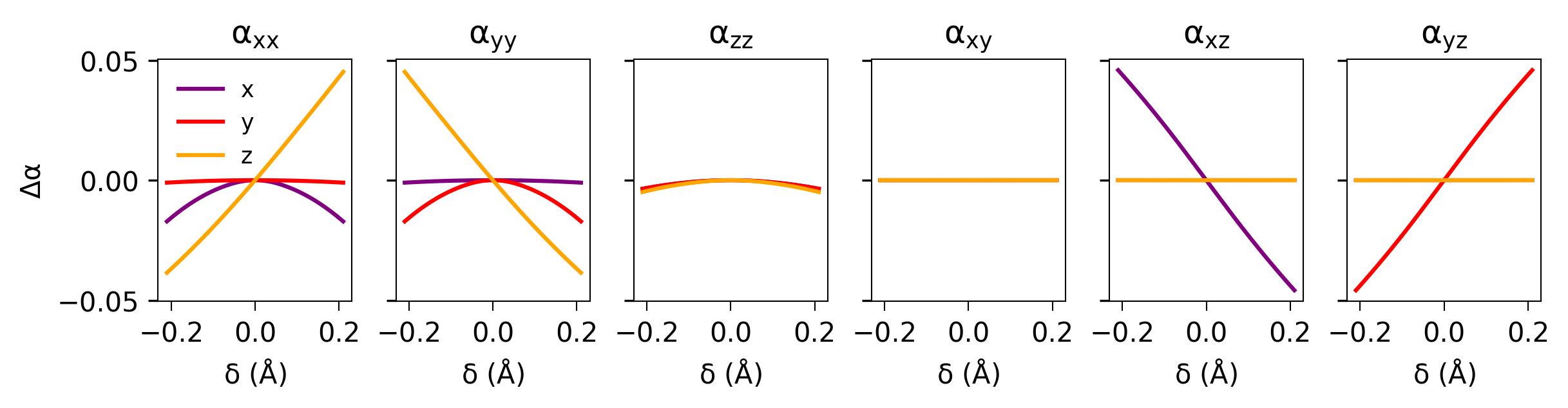
Just for fun, let’s visualize the interpolations for a specific atom.

atom_number = 5 # Feel free to change this!

fig = plt.figure(constrained_layout = True, figsize = (8, 2))
gs = fig.add_gridspec(1,6, wspace=0)
axes = gs.subplots(sharex=True, sharey=True)
interp_displacements = np.linspace(-0.21,0.21,50)

target_interps = []
signs = []
for direction_i in [0,1,2]:
    basis_vector = model.cart_basis_vectors[0] * 0
    basis_vector[atom_number-1][direction_i] = 1
    for basis, interp in zip(model.cart_basis_vectors,model._interpolations):
        if np.dot(basis.flatten(), basis_vector.flatten()) < -0.9:
            target_interps.append(interp)
            signs.append(-1)
        elif np.dot(basis.flatten(), basis_vector.flatten()) > 0.9:
            target_interps.append(interp)
            signs.append(1)


for axis_i, (i,j) in enumerate([(0,0),(1,1),(2,2),(0,1),(0,2),(1,2)]):
    axis = axes[axis_i] # type: ignore
    colors = ['purple', 'red', 'orange']
    labels = ['x','y','z']

    for interp,sign,color,label in zip(target_interps,signs,colors,labels):
        axis.plot(interp_displacements,
                  interp(sign*interp_displacements)[:,i,j], color = color, label = label)
    axis.set_xlabel(r"$\delta$ (Å)")
    subscripts = ['x','y','z']
    alpha_string = r"$\alpha_{" + subscripts[i] + subscripts[j] + "}$"
    axis.set_title(alpha_string)
    if axis_i == 0:
        l = axis.legend(fontsize = "small", frameon = False)

l = axes[0].set_ylabel(r"$\Delta\alpha$")

Calculating a Raman spectrum

With the model specified, we’re ready to calculate a Raman spectrum.

# Compute and plot spectrum
spectrum = phonons.get_raman_spectrum(model)
wavenumbers, intensities = spectrum.measure(laser_correction = True,
                                           laser_wavelength = 532,
                                           bose_einstein_correction = True,
                                           temperature = 300)
fig = plt.figure(constrained_layout = True, figsize = (8, 3))
axis = fig.add_subplot(111)
axis.plot(wavenumbers, intensities)
axis.set_ylabel("Intensity (a.u.)")
l = axis.set_xlabel(r"Raman shift ($\mathregular{cm^{-1}}$)")

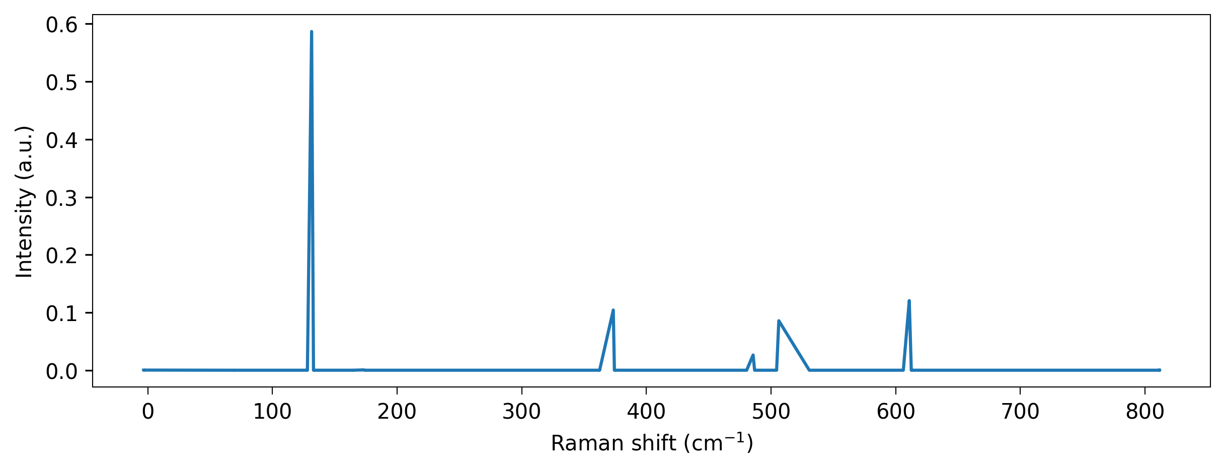
spectrum.calculate returns a fairly unprocessed spectrum - literally a list of phonon frequencies and intensities. To make a nicer, more realistic visualization, we can broaden the spectra through convolutions.

# Let's make it prettier.
wavenumbers, intensities = spectrum.measure(laser_correction = True,
                                laser_wavelength = 532,
                                           bose_einstein_correction = True,
                                           temperature = 300)
wavenumbers, intensities = rn.spectrum.utils.convolve_spectrum(wavenumbers, intensities)

fig = plt.figure(constrained_layout = True, figsize = (8, 3))
axis = fig.add_subplot(111)
axis.plot(wavenumbers, intensities)
axis.set_ylabel("Intensity (a.u.)")
l = axis.set_xlabel(r"Raman shift ($\mathregular{cm^{-1}}$)")

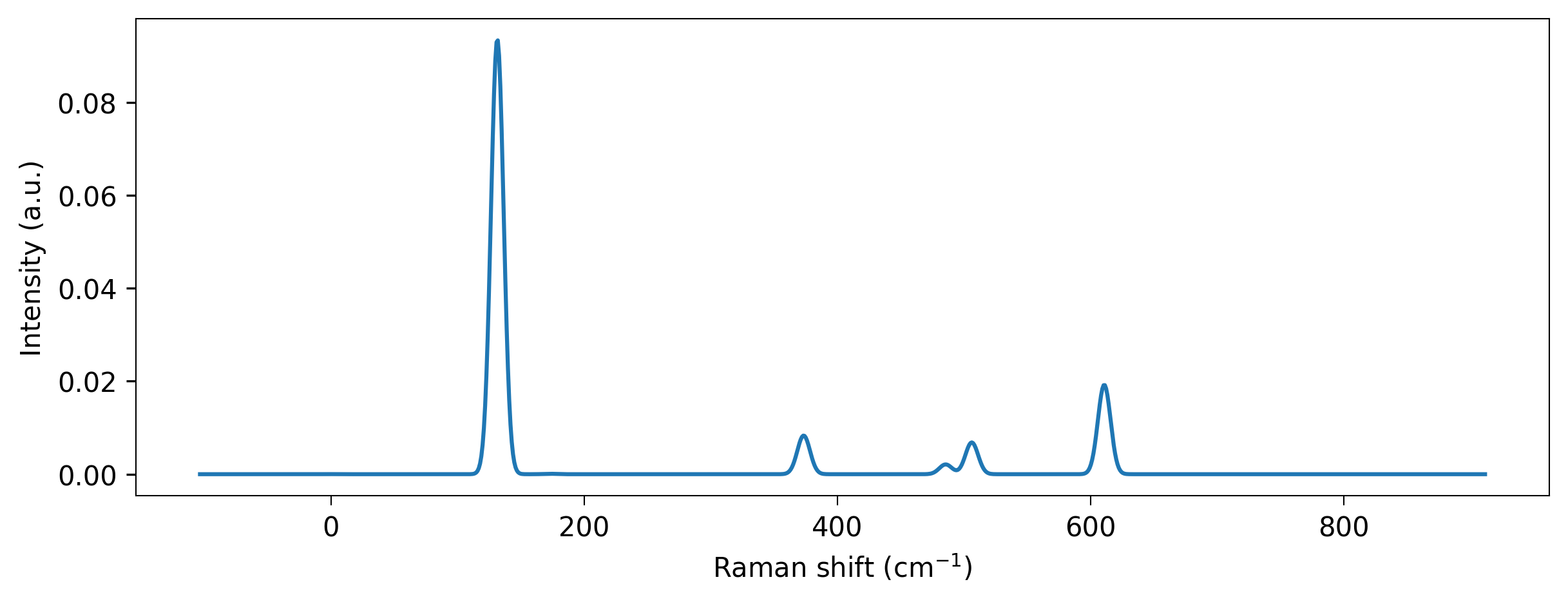
And there you have it! Using ramannoodle’s InterpolationModel, we calculated a full Raman spectrum for TiO2 using data from just a handful of polarizability calculations.

Next, we will introduce ARTModel and give a more complete overview of ramannoodle’s workflow: Full workflow